Loss Types
Real measurements contain noise, and often a few points that are simply wrong.
The loss_type parameter controls how hard a residual is allowed to pull on the
fitted surface:
loss_type |
Behavior | Use when |
|---|---|---|
'rmse' |
Squared error — every residual pulls with its full weight | Data is clean |
'huber' |
Quadratic core, linear tails — outlier pull is capped | Data is noisy (recommended default) |
'tukey' |
Redescending — residuals past the rejection point pull with zero force | Some points are outright erroneous |
The Shape of Each Loss
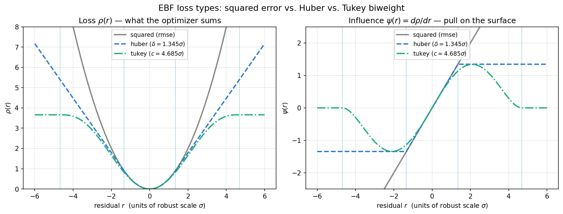
The left panel is \(\rho(r)\), the penalty each residual contributes. The right panel is the influence \(\psi(r) = d\rho/dr\) — how hard a point at that residual actually pulls on the surface. The influence curve is the one that matters for robustness:
- Squared error influence grows without bound. A point twice as far away pulls twice as hard, so a single bad measurement can dominate the fit.
- Huber influence is clipped beyond \(\delta\). Outliers still pull, but with a constant, bounded force no matter how wrong they are (ADR-009/013).
- Tukey biweight influence redescends to exactly zero beyond \(c\). Points out there are effectively deleted from the problem (ADR-014).
Thresholds are drawn at the classical tuning constants used by the 'auto'
calibration: \(\delta = 1.345\sigma\) and \(c = 4.685\sigma\), where \(\sigma\) is a
robust estimate of the residual scale. Both retain roughly 95% of the
efficiency of least squares on clean Gaussian data.
Regenerate this figure with
examples/loss_function_gallery.py.
Behavior on Real Data
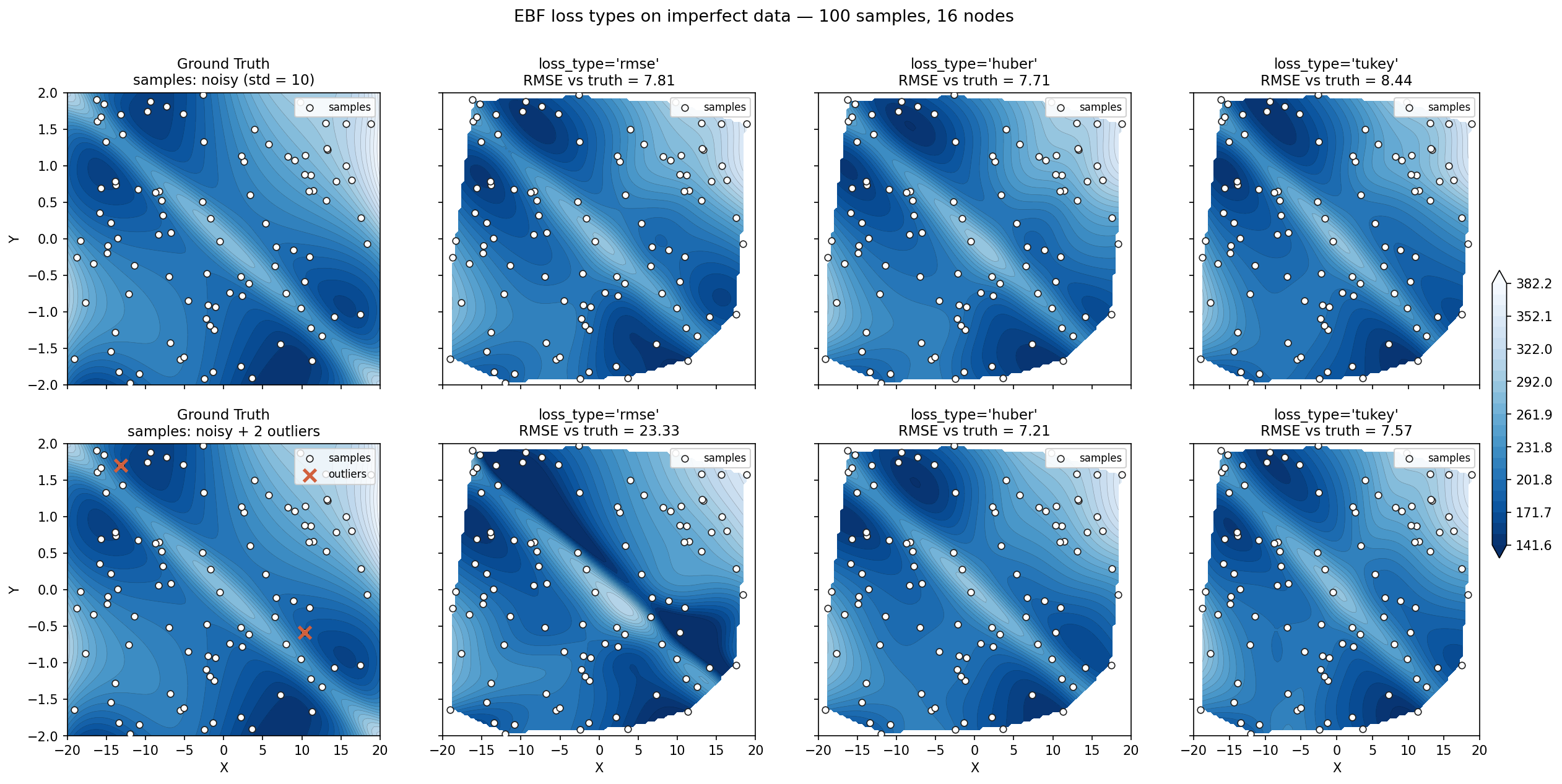
The shapes above predict what happens to a fit, but the effect is easier to see directly. Below, the same 2-D test surface is sampled 100 times and fit with all three losses under two corruption scenarios — each fit scored against the clean ground truth, so the numbers measure how well the underlying surface was recovered.
| Scenario | rmse |
huber |
tukey |
|---|---|---|---|
| Noisy (std = 10) | 7.81 | 7.71 | 8.44 |
| Noisy + 2 gross outliers | 23.33 | 7.21 | 7.57 |
Two things to take from this:
Noise alone is not the problem. With only Gaussian noise, all three losses land within about 10% of each other. Tukey trails slightly — its aggressive rejection also discards genuine sharp features along the diagonal ridge, which is the cost of redescending influence.
Gross outliers are. Adding just two bad points out of 100 triples the squared-error RMSE and tears a visible gash across the surface, because those two residuals pull harder than everything else combined. Both robust losses absorb them and hold near 7.2.
Regenerate with
examples/loss_comparison.py.
Choosing Between Huber and Tukey
Start with 'huber'. In the comparison above it was at least as good as
Tukey in both scenarios, and it degrades gracefully — a mis-set threshold costs
a little accuracy rather than silently discarding good data.
Reach for 'tukey' when outliers are numerous or extreme enough that even
Huber's bounded linear pull still drags the surface. Because Tukey's influence
returns to zero, its total contribution from bad points is finite no matter how
many there are. Raising n_outliers or outlier_size in
examples/loss_comparison.py shows it taking the lead.
Tukey is non-convex
A fixed, small tukey_c can reject most of the data at initialization and
stall training before it starts. Prefer an adaptive setting — 'auto' or a
'<k>sigma' spec — which anneals from an effectively quadratic start as the
residual scale tightens.
Adaptive Thresholds
Both huber_delta and tukey_c default to 'auto' and are expressed in
scaled data space, not your original units — the model standardizes inputs
and outputs internally.
With 'auto', the threshold is recalibrated every 100 steps from a robust
(median-absolute-deviation) estimate of the current residual spread. This
matters because the right threshold at step 0, when the surface is still far
from the data, is very different from the right threshold at convergence. As
the fit tightens, the threshold tracks it down.
Each parameter accepts three forms:
| Value | Threshold | Adapts during training? |
|---|---|---|
'auto' (default) |
\(K_\text{default}\,\hat\sigma\) — \(1.345\hat\sigma\) for Huber, \(4.685\hat\sigma\) for Tukey | Yes |
'2.5sigma' |
\(2.5\,\hat\sigma\) — your tuning constant | Yes |
0.8 |
fixed at 0.8, in scaled data space | No |
model.fit(X, y, loss_type='huber', huber_delta='auto')       # recommended
model.fit(X, y, loss_type='huber', huber_delta='1.0sigma')   # adaptive, custom K
model.fit(X, y, loss_type='huber', huber_delta=0.8)          # fixed threshold
The spec is whitespace- and *-tolerant: '3sigma', '3 sigma', and
'3 * sigma' are all the same thing. '1.345sigma' is exactly equivalent to
'auto' for Huber.
Choosing K
\(K\) sets the trade-off between efficiency on clean Gaussian noise and resistance to contamination. Lower \(K\) downweights more aggressively.
| Loss | Default \(K\) | More aggressive | Effect |
|---|---|---|---|
'huber' |
1.345 (95% efficiency, ~18% of points in the linear zone) | '1.0sigma' |
More residuals treated linearly — use under heavy contamination |
'tukey' |
4.685 (95% efficiency) | '3sigma' |
Rejects considerably more; a common choice when outliers are numerous |
Below about \(K = 2\) for Tukey the annealing argument starts to break down and
training can stall, for the same reason a small fixed c does.
Pass a float only when you have a specific reason to pin the threshold in absolute terms — e.g. you know the instrument's noise floor in scaled units and want it held there regardless of how the fit evolves.
Note
huber_delta is only read when loss_type='huber', and tukey_c only when
loss_type='tukey'. Setting one while using the other loss has no effect.
Related
- Visualization — the residual plot is the quickest way to judge whether a robust loss is warranted
- Algorithm Overview — where the loss sits in training
- Decisions — ADR-009, ADR-013, ADR-014