Example: RBF vs EBF

This is the headline comparison — what EBF buys you over a conventional radial basis function fit. The full script is at examples/RBF_vs_EBF.py.

The Test Surface

The surface is built to stress an isotropic kernel: a smooth polynomial swell plus a narrow ridge running diagonally across the domain.

def test_func(x, y):
    xn = x / 10.0
    base  = (xn**5 + 3*xn*y + 1.5*y**2 + 5) * (xn + y) + 200 + np.sin(xn * y) * 50
    ridge = 80 * np.exp(-10 * (xn + y)**2)
    return base + ridge

An isotropic kernel has a single length scale in every direction. To resolve a narrow ridge it must shrink that length scale everywhere — which then leaves it under-constrained between samples in the smooth directions. The result is ringing.

The domain is deliberately 40 × 4 (a 10:1 aspect ratio). EBF's internal standardization handles this; scipy's Rbf sees the raw coordinates.

The Comparison

Both methods see the same 50 scattered samples.

# EBF — 16 learned nodes
model = ebf.EBF(n_nodes=16, basis='multiquadric')
model.fit(
    X_pts, z_pts,
    steps=60000,
    loss_threshold=0.04,     # stop early once the loss is good enough
    var_weight=0.01,         # light node-spread regularization
    ellipsoid_weight=0.001,  # light smoothness penalty (ADR-011)
    loss_type='huber',
    huber_delta='auto',
    seed=42,
)

# Scipy RBF — exact interpolation, one center per sample (50 of them)
rbfi = Rbf(X_pts[:, 0], X_pts[:, 1], z_pts, function='multiquadric')

Note the asymmetry, which favors the baseline: the RBF gets a center at every sample, while EBF is restricted to 16 nodes.

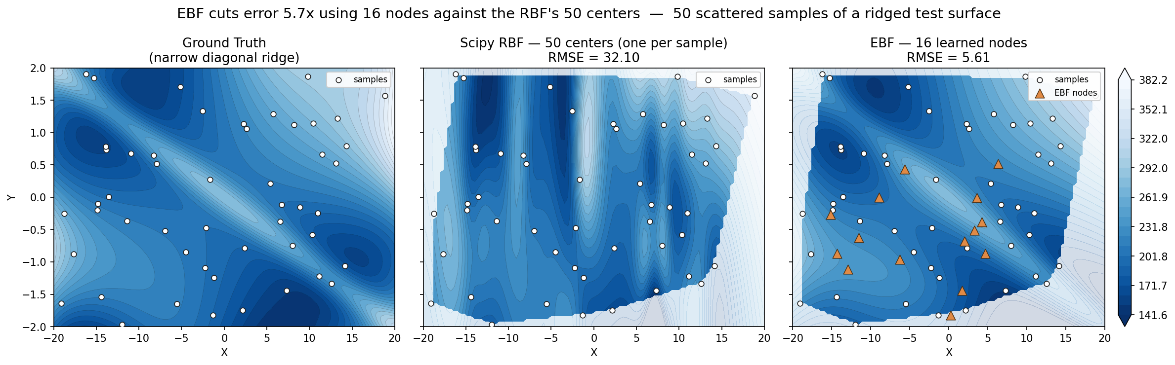
Method	Centers / nodes	RMSE vs ground truth
Scipy RBF (multiquadric)	50	32.10
EBF (multiquadric)	16	5.61

EBF cuts the error by a factor of 5.7 using roughly a third as many centers. The RBF panel shows the characteristic failure: vertical striping as the isotropic kernel rings around a feature it cannot align with.

Scoring Fairly

Both methods extrapolate freely outside the sample hull, and comparing them out there measures extrapolation behavior rather than fit quality. The script masks to the convex hull of the training points and scores only inside it:

outside = hull_mask(X_pts, xx, yy)
inside = ~outside
rmse_ebf = np.sqrt(np.mean((z_ebf[inside] - z_true[inside]) ** 2))

The faint regions outside the hull in the figure are that extrapolation, drawn at low opacity for context but excluded from the numbers.

Why It Works

Each EBF node carries its own positive-definite matrix that the optimizer may stretch and rotate, so a node sitting on the ridge can elongate along it.

On this fit the learned ellipsoids align with the ridge to a median of 4.4 degrees, with 12 of the 16 nodes within 15 degrees of it. They also become extremely elongated — aspect ratios reach the tens of thousands — which is why they are not drawn on the figure above: at r = 1 each contour degenerates into a pair of near-parallel lines spanning the whole domain.

For a legible picture of the same mechanism, see examples/node_ellipsoids.py, which uses 3 nodes and a decaying basis so the ellipses stay compact:

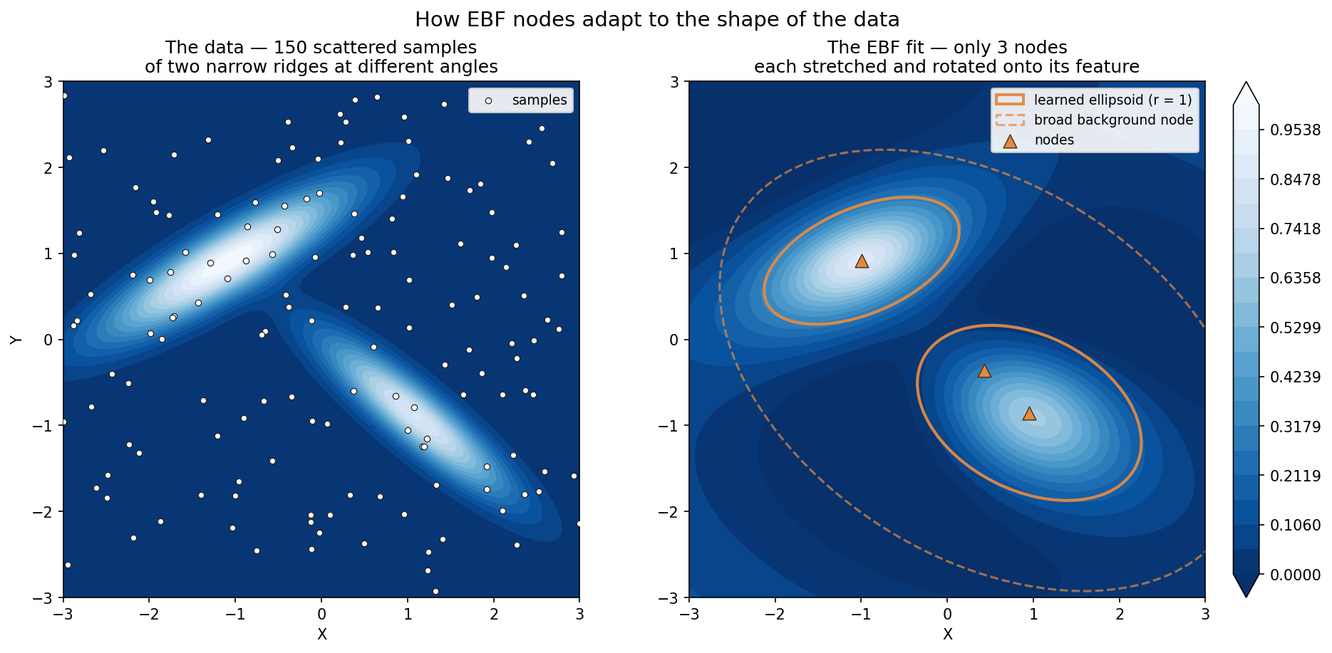
Ellipsoid shape depends on the basis family

Growing bases (multiquadric, matern52) tend toward slab-like ellipsoids. Decaying bases (gaussian, inv_quadratic) keep them compact enough to plot. Check with EBF.get_ellipsoids() before trying to draw them.

Reproducing

python examples/RBF_vs_EBF.py

The figure is written to docs/assets/rbf_vs_ebf.png. Pass --save-only to skip the interactive window, or regenerate every documentation figure at once:

python examples/make_docs_figures.py