Basis Functions

The basis function determines how each node's influence changes with distance. EBF provides 12 basis functions, selected by passing a string name to the basis parameter:

model = ebf.EBF(n_nodes=10, basis='gaussian')

Gallery

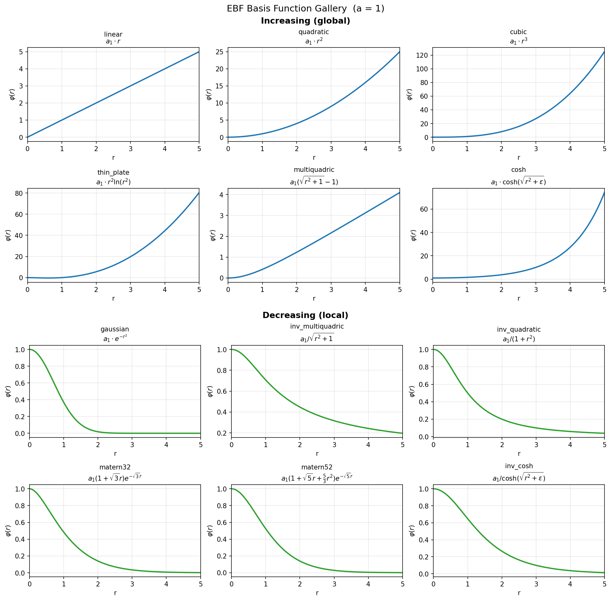
The chart below shows all basis functions evaluated with unit weight (\(a_1 = 1\)) over a range of radii.

Reference Table

Growing Functions

These functions increase without bound as distance grows. They produce smooth surfaces that can extrapolate beyond the data range (for better or worse).

Name	Expression	When to Use
linear	\(a_1 \cdot r\)	Simple problems; piecewise-linear feel
quadratic	\(a_1 \cdot r^2\)	Smooth parabolic influence
cubic	\(a_1 \cdot r^3\)	Very smooth; similar to natural splines
multiquadric	\(a_1 (\sqrt{r^2+1} - 1)\)	Default. Good general choice; grows sub-linearly
cosh	\(a_1 \cdot \cosh(\sqrt{r^2+\varepsilon})\)	Exponential growth at large \(r\); use with care

Decaying Functions

These functions decay toward zero at large distances. Nodes have localized influence — far-away nodes don't affect the prediction. Good when you want the model to avoid wild extrapolation outside the data hull.

Name	Expression	When to Use
gaussian	\(a_1 \cdot e^{-r^2}\)	Classic localized influence; decays very quickly
inv_multiquadric	\(a_1 / \sqrt{r^2+1}\)	Complement to multiquadric; gentle decay
inv_quadratic	\(a_1 / (1+r^2)\)	Cauchy-like; heavier tails than Gaussian
inv_cosh	\(a_1 / \cosh(\sqrt{r^2+\varepsilon})\)	Sech-like decay; complement to cosh
matern32	\(a_1 (1+\sqrt{3}r) e^{-\sqrt{3}r}\)	C1-smooth; popular for physical/engineering data
matern52	\(a_1 (1+\sqrt{5}r+\frac{5}{3}r^2) e^{-\sqrt{5}r}\)	C2-smooth; smoother than Matern 3/2

Special Functions

These have logarithmic behavior near zero.

Name	Expression	When to Use
thin_plate	\(a_1 \cdot r^2 \ln(r^2)\)	Classic thin-plate spline; C1 smooth

Choosing a Family: the Node-Count Tradeoff

The growing/decaying split is usually presented as a question about extrapolation — and it is, but it also decides how forgiving the basis is about n_nodes.

The two families fail differently when given surplus capacity:

• Growing bases increase with distance, so every node influences every point. Local features are built by cancellation between nodes, and there is no way to raise a private spike over a single data point. Surplus nodes go into near-collinear directions that leave the surface smooth.
• Decaying bases fall to zero with distance, so each node owns a neighborhood and is a local feature in its own right. As the node count approaches the sample count, each node can sit on a point and chase its noise.

examples/node_count_gallery.py sweeps a representative of each family from 4 nodes to one node per sample — 256 samples of a ridged surface with 5% noise (\(\sigma = 2.11\)), trained to convergence at 80,000 steps. The rightmost column is 1539 parameters against 256 observations.

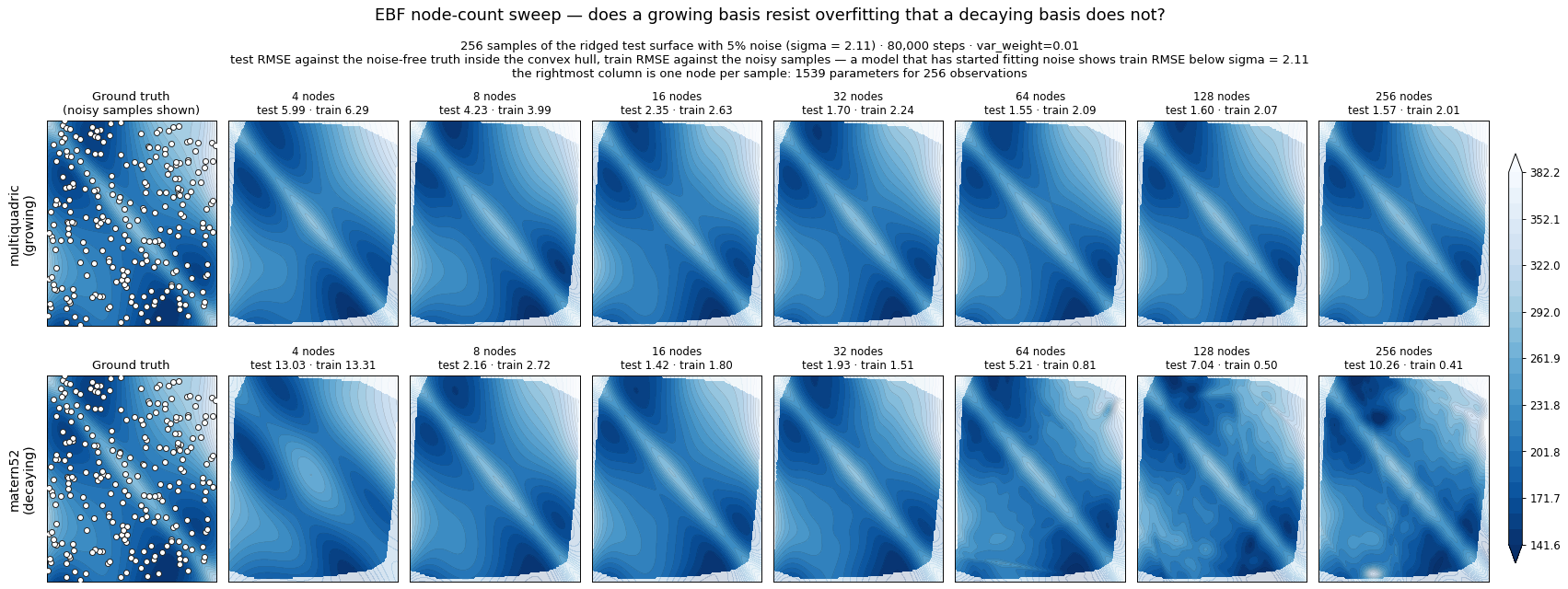
The top row barely changes past 32 nodes. The bottom row visibly breaks up from 64 nodes onward — those blotches are nodes sitting on individual samples and chasing their noise.

basis	family	best test RMSE	at 256 nodes	penalty	train RMSE at 256
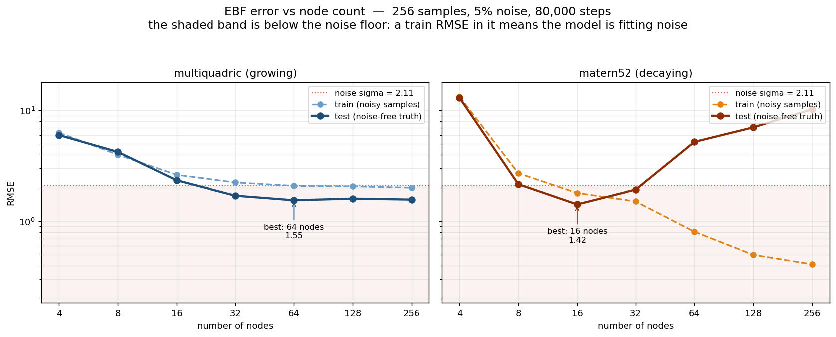
multiquadric	growing	1.55 (64 nodes)	1.57	1.01×	2.01 — at the noise floor
matern52	decaying	1.42 (16 nodes)	10.26	7.2×	0.41 — a fifth of \(\sigma\)

The growing basis is essentially flat once it has enough nodes. The decaying basis has a sharp optimum and degrades hard past it, and its training error keeps falling below the noise floor the whole way — the signature of a model fitting noise rather than signal.

Two conditions, both easy to miss

A decaying basis turns early — well before one node per sample. matern52 is already past its optimum at 32 nodes (ratio 0.125) and 3.4× worse by 64. The blowup at the far end is the dramatic version, but the damage starts much sooner than "extreme" would suggest.

The model has to actually reach capacity. Gradient descent from a small initialization over a finite step budget is itself a regularizer, and a model that stopped before fitting the signal cannot demonstrate anything about overfitting — at a short step budget both families look equally well behaved. Read training RMSE against the noise floor: a model chasing noise sits below \(\sigma\). If it sits above, you are measuring how far Adam got, not what the node count does.

What to do with this:

• With the default multiquadric — or any growing basis — the usual guidance of n_nodes at 1/3 to 1/2 your point count holds, and erring high is cheap. This is the main reason it is the default.
• With a decaying basis that rule does not hold: at 1/3 of 256 points matern52 is already ~5× worse than its best. Start lower, around 1/10 of your point count, and tune upward while watching held-out error rather than training error.
• Either way, compare training RMSE against your expected noise level. Setting val_fraction=0.15 catches this automatically.

Scope of this measurement

One synthetic 2-D surface, one noise level, and two of the twelve basis functions — chosen as clear representatives of each family. Each node costs \(1 + n_{dims} + n_{dims}(n_{dims}+1)/2\) parameters, so how fast you reach the over-parameterized regime is dimension-dependent, and the node counts above will not transfer directly to your data. Treat the direction as the finding, and the specific crossover point as something to check on your own held-out set.

Notes

• \(r\) is the non-Euclidean distance from the input point to a node (not the squared distance). In the code, the basis functions receive \(r^2\) directly and compute \(r\) internally where needed.

• \(\varepsilon\) is a small numerical stability offset (default 1e-8), set via the eps parameter on the EBF constructor. Only cosh and inv_cosh use it. thin_plate uses tf.math.xlogy which handles the \(r = 0\) case natively. All other functions have no singularity at \(r = 0\).