How the Algorithm Works

This page explains the EBF algorithm in plain language. You don't need to be a mathematician to follow it — just a technical user comfortable with concepts like "distance", "weights", and "optimization".

The Big Picture

Imagine you have a handful of measurements scattered across a 2D space — say, compressor efficiency at various combinations of mass flow and pressure ratio. You want to draw a smooth surface through those points so you can estimate efficiency at locations you haven't measured.

EBF does this by placing nodes in the input space. Each node acts like a little hill (or valley) of influence. The model's prediction at any point is the weighted sum of contributions from all nodes, plus a simple linear trend. During training, the optimizer adjusts everything — node positions, influence shapes, and weights — to minimize the prediction error.

Nodes and Influence Zones

In a standard Radial Basis Function (RBF), each node measures distance using ordinary Euclidean distance — a circle in 2D, a sphere in 3D. Every node uses the same distance metric.

EBF replaces that circle with an ellipse (or ellipsoid in higher dimensions). Each node gets its own ellipse that the optimizer can stretch and rotate independently. This means:

• A node near a steep gradient can stretch its influence along the contour (where values change slowly) and shrink it across the gradient (where values change quickly).
• Different nodes can have completely different shapes and orientations.

This is the "elliptical" in Elliptical Basis Function — it's the key generalization over standard RBF.

How the ellipse is built: Each node stores a small matrix (called L). The actual ellipse shape comes from multiplying L by its transpose (L x L^T). This mathematical trick guarantees the ellipse is always valid (positive-definite) no matter what values the optimizer puts in L. No special constraints or penalty terms are needed during training.

How a Prediction is Made

When you call model.predict(X), here's what happens for each input point:

1. Measure distances — For each node, compute the "elliptical distance" from the input point to that node. This uses the node's custom ellipse shape, not plain Euclidean distance. The result: one distance value per node.

2. Apply the basis function — Feed each distance through a nonlinear function (the "basis function"). The default is the multiquadric function, which grows slowly with distance. This converts each distance into a contribution value.

3. Weighted sum — Multiply each node's contribution by its learned weight (a1), then sum them all up. This gives the RBF part of the prediction.

4. Add the linear trend — Add a simple slope * input + intercept term. This captures any global trend in the data (e.g., efficiency generally increasing with flow rate), so the nodes only need to model the residual wiggles.

5. Output — The sum of the RBF contribution and the linear trend is the final prediction.

In short: distance → basis function → weighted sum → add trend → output.

How the Model Learns

All parameters are trained simultaneously using gradient descent (the Adam optimizer). "All parameters" means:

• Node positions — where each node sits in input space
• Ellipsoid shapes — how each node's influence zone is stretched and rotated
• Amplitude weights (a1, and a2/a3 for some basis functions) — how much each node contributes to the output
• Linear trend (b1, b2) — the slope and intercept of the global trend

The loss function has up to three parts:

1. Prediction error (RMSE or Huber loss) — By default, EBF uses RMSE (root-mean-square error). For noisy data, you can switch to Huber loss with loss_type='huber'. Huber loss behaves quadratically for small residuals (like RMSE) but switches to linear for residuals larger than huber_delta. This makes the model robust to noisy outliers — a single bad measurement won't warp the entire surface toward it. RMSE squares every residual, so a point that's 10x noisier than the rest becomes 100x more influential. Huber caps that influence at 10x.

By default (huber_delta='auto') the threshold is recalibrated every 100 steps from the spread of the current residuals (a robust median-based estimate that outliers cannot corrupt), so it tracks the noise floor as the fit tightens and roughly the largest ~18% of residuals get the linear, outlier-resistant treatment. The Huber term is also reported on the same scale as RMSE (it equals RMSE exactly when no residual exceeds the threshold), so loss_threshold and the regularization weights don't need retuning when you switch loss types.

For data containing erroneous points (bad sensor readings) rather than merely noisy ones, loss_type='tukey' goes further: the Tukey biweight is a redescending loss whose pull on the surface drops smoothly to exactly zero for residuals beyond the rejection point tukey_c — gross outliers are effectively discarded rather than just downweighted. Rejection is continuously reconsidered: if the surface later moves back toward a rejected point, that point regains its influence. The default tukey_c='auto' (recommended) tracks the residual noise floor at 4.685·σ with the same recalibration cadence and RMSE-comparable scaling; starting from an effectively quadratic state and tightening gradually also keeps the (non-convex) loss from rejecting good data early in training.

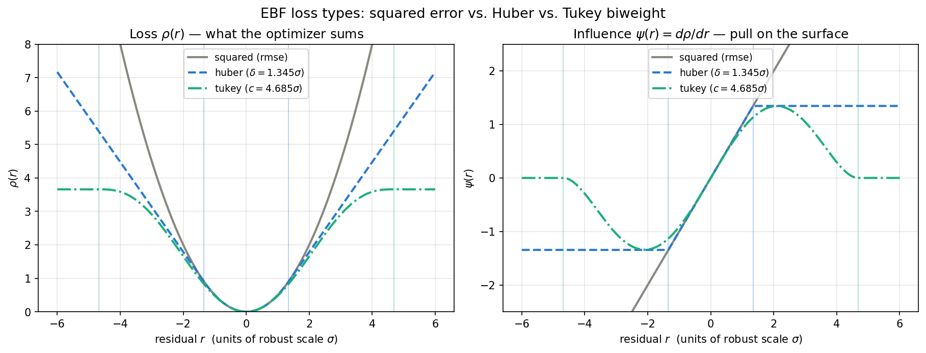
The left panel shows the per-point loss ρ(r): squared error grows without bound, Huber switches to linear growth beyond δ, and Tukey flattens to a constant beyond c. The right panel shows what actually matters to the optimizer — the influence ψ(r) = dρ/dr, the force with which a point of a given residual pulls on the surface. Squared error lets an outlier pull arbitrarily hard, Huber caps the pull at a constant, and Tukey's pull redescends to exactly zero: a point beyond the rejection point cannot move the surface at all. (The figure is generated by examples/loss_function_gallery.py; residuals are in units of the robust scale σ that the 'auto' thresholds are calibrated against.)

1. Node spread regularization — a penalty that increases sharply when nodes cluster together. Without it, the optimizer can fall into a trap where all nodes collapse to the same location (since a single-node model is a valid local minimum — just a bad one). The penalty ensures nodes stay spread out across the data. The var_weight parameter controls how strongly this penalty is applied.

var_weight also acts as a de facto smoothing parameter, and in practice it works well in this role. The mechanism is indirect but consistent: forcing nodes apart means each node ends up farther from the data points it is responsible for. To still fit the data accurately, the optimizer responds by scaling down the non-Euclidean distances — effectively making each node's ellipsoid "reach farther" so that its basis-function response (the r value) stays in a moderate, well-behaved range. The result is that each node exerts a broader, more diffuse influence across the input space, which produces a smoother surface. Higher var_weight → more spread → broader influence zones → smoother fit. Conversely, very low var_weight allows nodes to cluster and punch narrow, high-amplitude bumps into the surface.

1. Ellipsoid shape penalty (optional) — activated with ellipsoid_weight (default 0 = off). It penalizes the overall magnitude of each node's ellipsoid matrix, which caps how sharp and narrow any node's influence zone can become. Sharp spikes in an EBF surface come from extreme ellipsoids, so this is the explicit smoothness knob: raise it (starting around 0.01) when the fit chases noise even after tuning var_weight. See ADR-011 in docs/design/DECISIONS.md.

Note there is deliberately no amplitude penalty. An L2 penalty on the per-node amplitudes (smooth_weight) was trialed and rejected — because the ellipsoid matrices are learnable, the optimizer can dodge the penalty by shrinking amplitudes and inflating ellipsoids, leaving the surface unchanged (or sharper). See ADR-010 in docs/design/DECISIONS.md. The ellipsoid shape penalty above is its replacement: it acts on the ellipsoids directly, where the sharpness actually lives, and the dodge that defeated the amplitude penalty makes this one more expensive, not less. Smoothness is otherwise controlled by var_weight, node count, and basis choice.

Training uses full-batch gradient descent — every data point is used in every optimizer step. This works well because EBF datasets are typically small (tens to thousands of points, not millions). The learning rate starts at a user-specified value and decays exponentially over the course of training.

For noisy data, training can also stop itself automatically: setting val_fraction (e.g. 0.15) holds out that fraction of the points as a validation set. The validation loss is checked every 100 steps, and once it stops improving for patience checks — the point where the model switches from learning the trend to memorizing noise — training stops and the weights from the best-validation step are kept. Training loss alone cannot detect this transition, because memorizing noise keeps lowering it. Validation splitting needs roughly 50+ points to give a stable signal; on smaller datasets rely on regularization instead. See ADR-012 in docs/design/DECISIONS.md.

Data Scaling

Real engineering data has dimensions with very different scales — mass flow in kg/s, pressure ratio as a dimensionless number around 1-3, efficiency as a fraction near 0.8. If fed directly to the optimizer, the large-scale dimensions would dominate the distance calculations.

EBF handles this automatically: before training, each dimension is standardized (subtract the mean, divide by the standard deviation). After training, predictions and node positions are converted back to the original scale. You never need to scale your data manually.

Note

The scaling parameters (called Scale and Offset) are saved alongside the model weights. A model checkpoint without them cannot produce correct predictions.

Basis Functions

The basis function is the nonlinear function applied to each node's distance. Different basis functions produce different surface shapes. EBF ships with 15 options — from the default multiquadric (grows slowly, good general choice) to Gaussian (decays to zero, localized influence) to Matern kernels (popular in geostatistics).

See the Basis Functions page for the full gallery and guidance on when to use each one.